CLI Quick Start
This page explains how to train, evaluate, analyze, generate predictions, and measure the inference speed of a binary classification model using the CLI API.
An end-to-end example is available here.
Install YDF CLI
1. Go to the YDF GitHub Github release page.
2. Download the latest CLI release for your operating system. For example, to download the CLI release for Linux, click the "Download" button next to the "cli_linux.zip" file.
3. Extract the ZIP file to a directory of your choice e.g. unzip
cli_linux.zip.
4. Open a terminal window and navigate to the directory where you extracted the ZIP file.
Each executable (e.g. train, evaluate) executes a different task. For
example, the train command trains a model.
Each command is explained in the command page, or using the
--help flag:
Download dataset
For this example, we use the UCI Adult dataset. This dataset is a binary classification dataset, where the goal is to predict whether an individual's income is greater than $50,000. The features in the dataset are a mix of numerical and categorical.
First, we download a copy of the dataset from the UCI Machine Learning Repository:
DATASET_SRC=https://raw.githubusercontent.com/google/yggdrasil-decision-forests/main/yggdrasil_decision_forests/test_data/dataset
wget -q ${DATASET_SRC}/adult_train.csv -O adult_train.csv
wget -q ${DATASET_SRC}/adult_test.csv -O adult_test.csv
The first 3 examples of the training dataset are:
$ head -n 4 adult_train.csv

age,workclass,fnlwgt,education,education_num,marital_status,occupation,relationship,race,sex,capital_gain,capital_loss,hours_per_week,native_country,income
44,Private,228057,7th-8th,4,Married-civ-spouse,Machine-op-inspct,Wife,White,Female,0,0,40,Dominican-Republic,<=50K
20,Private,299047,Some-college,10,Never-married,Other-service,Not-in-family,White,Female,0,0,20,United-States,<=50K
40,Private,342164,HS-grad,9,Separated,Adm-clerical,Unmarried,White,Female,0,0,37,United-States,<=50K
The dataset is stored in two CSV files, one for training and one for testing. YDF can load CSV files directly, making it a convenient way to use this dataset.
When passing a dataset path to a command, the format of the dataset is always
specified using a prefix. For example, the prefix csv: in the path
csv:/path/to/my/file indicates that the file is a csv file. See
here
for the list of supported dataset formats.
Create dataspec
A dataspec (short for dataset specification) is a description of a dataset. It includes a list of available columns, the semantic (or type) of each column, and any other meta-data such as dictionaries or the rate of missing values.
The dataspec can be computed automatically using the infer_dataspec command
and stored in a dataspec file.
Looking at the dataspec before training a model is a great way to detect issues in the dataset, such as missing values, or incorrect data types.
The result is:
Number of records: 22792
Number of columns: 15

Number of columns by type:
    CATEGORICAL: 9 (60%)
    NUMERICAL: 6 (40%)

Columns:

CATEGORICAL: 9 (60%)
    3: "education" CATEGORICAL has-dict vocab-size:17 zero-ood-items most-frequent:"HS-grad" 7340 (32.2043%)
    14: "income" CATEGORICAL has-dict vocab-size:3 zero-ood-items most-frequent:"<=50K" 17308 (75.9389%)
    5: "marital_status" CATEGORICAL has-dict vocab-size:8 zero-ood-items most-frequent:"Married-civ-spouse" 10431 (45.7661%)
    13: "native_country" CATEGORICAL num-nas:407 (1.78571%) has-dict vocab-size:41 num-oods:1 (0.00446728%) most-frequent:"United-States" 20436 (91.2933%)
    6: "occupation" CATEGORICAL num-nas:1260 (5.52826%) has-dict vocab-size:14 num-oods:1 (0.00464425%) most-frequent:"Prof-specialty" 2870 (13.329%)
    8: "race" CATEGORICAL has-dict vocab-size:6 zero-ood-items most-frequent:"White" 19467 (85.4115%)
    7: "relationship" CATEGORICAL has-dict vocab-size:7 zero-ood-items most-frequent:"Husband" 9191 (40.3256%)
    9: "sex" CATEGORICAL has-dict vocab-size:3 zero-ood-items most-frequent:"Male" 15165 (66.5365%)
    1: "workclass" CATEGORICAL num-nas:1257 (5.51509%) has-dict vocab-size:8 num-oods:1 (0.0046436%) most-frequent:"Private" 15879 (73.7358%)

NUMERICAL: 6 (40%)
    0: "age" NUMERICAL mean:38.6153 min:17 max:90 sd:13.661
    10: "capital_gain" NUMERICAL mean:1081.9 min:0 max:99999 sd:7509.48
    11: "capital_loss" NUMERICAL mean:87.2806 min:0 max:4356 sd:403.01
    4: "education_num" NUMERICAL mean:10.0927 min:1 max:16 sd:2.56427
    2: "fnlwgt" NUMERICAL mean:189879 min:12285 max:1.4847e+06 sd:106423
    12: "hours_per_week" NUMERICAL mean:40.3955 min:1 max:99 sd:12.249

Terminology:
    nas: Number of non-available (i.e. missing) values.
    ood: Out of dictionary.
    manually-defined: Attribute which type is manually defined by the user i.e. the type was not automatically inferred.
    tokenized: The attribute value is obtained through tokenization.
    has-dict: The attribute is attached to a string dictionary e.g. a categorical attribute stored as a string.
    vocab-size: Number of unique values.
This example dataset contains 22,792 examples and 15 columns. There are 9 categorical and 6 numerical columns. The semantics of a column refers to the type of data it contains.
For example, the education column is a categorical column with 17 unique
possible values. The most frequent value is HS-grad (32% of all values).
(Optional) Create dataspec with a guide
In the example, the semantics of the columns were correctly detected. However, this might not be the case when the value representation is ambiguous. For example, the semantics of enum values (i.e., categorical values represented as an integer) cannot be automatically detected in a .csv file.
In such cases, we can re-run the infer_dataspec command with an extra flag to
indicate the real semantic of the miss-detected column. For example, to force
age to be detected as a numerical column, we would run:
# Force the detection of 'age' as numerical.
cat <<EOF > guide.pbtxt
column_guides {
    column_name_pattern: "^age$"
    type: NUMERICAL
}
EOF

./infer_dataspec --dataset=csv:adult_train.csv --guide=guide.pbtxt --output=dataspec.pbtxt
Train model
The model is trained with the train command. The label, features,
hyper-parameters and other training settings are specified in a training
configuration file.
# Create a training configuration file
cat <<EOF > train_config.pbtxt
task: CLASSIFICATION
label: "income"
learner: "GRADIENT_BOOSTED_TREES"
# Change learner-specific hyper-parameters.
[yggdrasil_decision_forests.model.gradient_boosted_trees.proto.gradient_boosted_trees_config] {
  num_trees: 500
}
EOF

# Train the model
./train \
  --dataset=csv:adult_train.csv \
  --dataspec=dataspec.pbtxt \
  --config=train_config.pbtxt \
  --output=model
Results:
[INFO train.cc:96] Start training model.
[INFO abstract_learner.cc:119] No input feature specified. Using all the available input features as input signal.
[INFO abstract_learner.cc:133] The label "income" was removed from the input feature set.
[INFO vertical_dataset_io.cc:74] 100 examples scanned.
[INFO vertical_dataset_io.cc:80] 22792 examples read. Memory: usage:1MB allocated:1MB. 0 (0%) examples have been skipped.
[INFO abstract_learner.cc:119] No input feature specified. Using all the available input features as input signal.
[INFO abstract_learner.cc:133] The label "income" was removed from the input feature set.
[INFO gradient_boosted_trees.cc:405] Default loss set to BINOMIAL_LOG_LIKELIHOOD
[INFO gradient_boosted_trees.cc:1008] Training gradient boosted tree on 22792 example(s) and 14 feature(s).
[INFO gradient_boosted_trees.cc:1051] 20533 examples used for training and 2259 examples used for validation
[INFO gradient_boosted_trees.cc:1434]   num-trees:1 train-loss:1.015975 train-accuracy:0.761895 valid-loss:1.071430 valid-accuracy:0.736609
[INFO gradient_boosted_trees.cc:1436]   num-trees:2 train-loss:0.955303 train-accuracy:0.761895 valid-loss:1.007908 valid-accuracy:0.736609
[INFO gradient_boosted_trees.cc:2871] Early stop of the training because the validation loss does not decrease anymore. Best valid-loss: 0.579583
[INFO gradient_boosted_trees.cc:230] Truncates the model to 136 tree(s) i.e. 136  iteration(s).
[INFO gradient_boosted_trees.cc:264] Final model num-trees:136 valid-loss:0.579583 valid-accuracy:0.870297
A few remarks:
-
Since no input features were specified, all columns except for the label are used as input features.
-
DFs natively consume numerical, categorical, and categorical-set features, as well as missing values. Numerical features do not need to be normalized, and categorical string values do not need to be encoded in a dictionary.
-
Except for the
num_treeshyperparameter, no training hyperparameters were specified. The default values of all hyperparameters are set such that they provide reasonable results in most situations. We will discuss alternative default values (called hyperparameter templates) and automated tuning of hyperparameters later. The list of all hyperparameters and their default values is available in the hyperparameters page. -
No validation dataset was provided for the training. Not all learners require a validation dataset. However, the
GRADIENT_BOOSTED_TREESlearner used in this example requires a validation dataset if early stopping is enabled (which is the case by default). In this case, 10% of the training dataset is used for validation. This rate can be changed using thevalidation_ratioparameter. Alternatively, the validation dataset can be provided with the--valid_datasetflag. The final model contains 136 trees for a validation accuracy of approximately 0.8702.
Show model information
Details about the model are shown with the show_model command.
Sample of the result:
Type: "GRADIENT_BOOSTED_TREES"
Task: CLASSIFICATION
Label: "income"

Input Features (14):
    age
    workclass
    fnlwgt
    education
    education_num
    marital_status
    occupation
    relationship
    race
    sex
    capital_gain
    capital_loss
    hours_per_week
    native_country

No weights

Variable Importance: MEAN_MIN_DEPTH:
    1.         "income"  4.868164 ################
    2.            "sex"  4.625136 #############
    3.           "race"  4.590606 #############
    ...
   13.     "occupation"  3.640103 ####
   14. "marital_status"  3.626898 ###
   15.            "age"  3.219872

Variable Importance: NUM_AS_ROOT:
    1.            "age" 28.000000 ################
    2. "marital_status" 22.000000 ############
    3.   "capital_gain" 19.000000 ##########
    ...
   11.  "education_num"  3.000000
   12.     "occupation"  2.000000
   13. "native_country"  2.000000

Variable Importance: NUM_NODES:
    1.     "occupation" 516.000000 ################
    2.            "age" 431.000000 #############
    3.      "education" 424.000000 ############
    ...
   12.  "education_num" 73.000000 #
   13.            "sex" 39.000000
   14.           "race" 26.000000

Variable Importance: SUM_SCORE:
    1.   "relationship" 3103.387636 ################
    2.   "capital_gain" 2041.557944 ##########
    3.      "education" 1090.544247 #####
    ...
   12.      "workclass" 176.876787
   13.            "sex" 49.287215
   14.           "race" 13.923084


Loss: BINOMIAL_LOG_LIKELIHOOD
Validation loss value: 0.579583
Number of trees per iteration: 1
Node format: BLOB_SEQUENCE
Number of trees: 136
Total number of nodes: 7384

Number of nodes by tree:
Count: 136 Average: 54.2941 StdDev: 5.7779
Min: 33 Max: 63 Ignored: 0
----------------------------------------------
[ 33, 34)  2   1.47%   1.47% #
...
[ 60, 62) 16  11.76%  96.32% ########
[ 62, 63]  5   3.68% 100.00% ##

Depth by leafs:
Count: 3760 Average: 4.87739 StdDev: 0.412078
Min: 2 Max: 5 Ignored: 0
----------------------------------------------
[ 2, 3)   14   0.37%   0.37%
[ 3, 4)   75   1.99%   2.37%
[ 4, 5)  269   7.15%   9.52% #
[ 5, 5] 3402  90.48% 100.00% ##########

Number of training obs by leaf:
Count: 3760 Average: 742.683 StdDev: 2419.64
Min: 5 Max: 19713 Ignored: 0
----------------------------------------------
[     5,   990) 3270  86.97%  86.97% ##########
[   990,  1975)  163   4.34%  91.30%
...
[ 17743, 18728)   10   0.27%  99.55%
[ 18728, 19713]   17   0.45% 100.00%

Attribute in nodes:
    516 : occupation [CATEGORICAL]
    431 : age [NUMERICAL]
    424 : education [CATEGORICAL]
    420 : fnlwgt [NUMERICAL]
    297 : capital_gain [NUMERICAL]
    291 : hours_per_week [NUMERICAL]
    266 : capital_loss [NUMERICAL]
    245 : native_country [CATEGORICAL]
    224 : relationship [CATEGORICAL]
    206 : workclass [CATEGORICAL]
    166 : marital_status [CATEGORICAL]
    73 : education_num [NUMERICAL]
    39 : sex [CATEGORICAL]
    26 : race [CATEGORICAL]

Attribute in nodes with depth <= 0:
    28 : age [NUMERICAL]
    22 : marital_status [CATEGORICAL]
    19 : capital_gain [NUMERICAL]
    12 : capital_loss [NUMERICAL]
    11 : hours_per_week [NUMERICAL]
    11 : fnlwgt [NUMERICAL]
    8 : relationship [CATEGORICAL]
    8 : education [CATEGORICAL]
    6 : race [CATEGORICAL]
    4 : sex [CATEGORICAL]
    3 : education_num [NUMERICAL]
    2 : native_country [CATEGORICAL]
    2 : occupation [CATEGORICAL]

...

Condition type in nodes:
    1844 : ContainsBitmapCondition
    1778 : HigherCondition
    2 : ContainsCondition
Condition type in nodes with depth <= 0:
    84 : HigherCondition
    52 : ContainsBitmapCondition
Condition type in nodes with depth <= 1:
    243 : HigherCondition
    165 : ContainsBitmapCondition
...
The structure of the tree of the model can be printed using the
--full_definition flag.
Evaluate model
The evaluation results are computed and printed as text (--format=text,
default) or as HTML with plots (--format=html) with the evaluate command.
# Evaluate the model and print the result in the console.
./evaluate --dataset=csv:adult_test.csv --model=model
Results
Evaluation:
Number of predictions (without weights): 9769
Number of predictions (with weights): 9769
Task: CLASSIFICATION
Label: income

Accuracy: 0.874399  CI95[W][0.86875 0.879882]
LogLoss: 0.27768
ErrorRate: 0.125601

Default Accuracy: 0.758727
Default LogLoss: 0.552543
Default ErrorRate: 0.241273

Confusion Table:
truth\prediction
       <OOD>  <=50K  >50K
<OOD>      0      0     0
<=50K      0   6971   441
 >50K      0    786  1571
Total: 9769

One vs other classes:
  "<=50K" vs. the others
    auc: 0.929207  CI95[H][0.924358 0.934056] CI95[B][0.924076 0.934662]
    p/r-auc: 0.975657  CI95[L][0.971891 0.97893] CI95[B][0.973397 0.977947]
    ap: 0.975656   CI95[B][0.973393 0.977944]

  ">50K" vs. the others
    auc: 0.929207  CI95[H][0.921866 0.936549] CI95[B][0.923642 0.934566]
    p/r-auc: 0.830708  CI95[L][0.815025 0.845313] CI95[B][0.817588 0.843956]
    ap: 0.830674   CI95[B][0.817513 0.843892]
Observations:
- The test dataset contains 9769 examples.
- The test accuracy is 0.874399 with 95% confidence interval boundaries of [0.86875; 0.879882].
- The test AUC is 0.929207 with 95% confidence interval boundaries of [0.924358 0.934056] when computed with a closed form and [0.973397 0.977947] when computed with bootstrapping.
- The PR-AUC and AP metrics are also available.
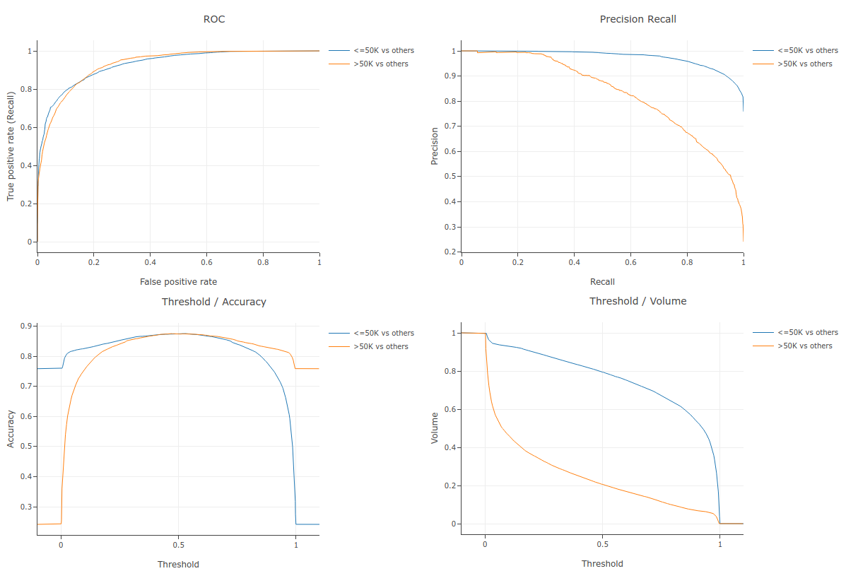
The following command evaluates the model and exports the evaluation report to an HTML file.
# Evaluate the model and print the result in an Html file.
./evaluate --dataset=csv:adult_test.csv --model=model --format=html > evaluation.html
Generate predictions
The predictions are computed and exported to file with the predict command.
# Exports the prediction of the model to a csv file
./predict --dataset=csv:adult_test.csv --model=model --output=csv:predictions.csv

# Show the predictions for the first 3 examples
head -n 4 predictions.csv
Results:
Benchmark model speed
In time-critical applications, the inference speed of a model can be crucial.
The benchmark_inference command measures the average inference time of the
model.
YDF has multiple algorithms to compute the predictions of a model. These algorithms differ in speed and coverage. When generating predictions, YDF automatically uses the fastest algorithm compatible.
The benchmark_inference shows the speed of all the compatible algorithms.
Inference algorithms are single-threaded, meaning that they can only process one data point at a time. It is up to the user to parallelize inference using multi-threading.
# Benchmark the inference speed of the model
./benchmark_inference --dataset=csv:adult_test.csv --model=model
Results:
batch_size : 100  num_runs : 20
time/example(us)  time/batch(us)  method
----------------------------------------
            0.89              89  GradientBoostedTreesQuickScorerExtended [virtual interface]
          5.8475          584.75  GradientBoostedTreesGeneric [virtual interface]
          12.485          1248.5  Generic slow engine
----------------------------------------
We see that the model can run a 0.89 µs (micro-seconds) per example on average.