Glossary
Bootstrapping
A way to estimate confidence intervals and statistical significance using
randomization. The confidence intervals and statistical significance of metrics
computed using Bootstrapping are tagged by [B]. Unless specified otherwise,
bootstrapping is non-parametric and runs at the "example/prediction" level.
Default metrics
A default metric (e.g., default accuracy) is the maximum possible value of a metric for a model always outputting the same value. For example, in a balanced binary classification dataset, the default accuracy is 0.5.
Classification
ACC (Accuracy)
The accuracy (Acc) is the ratio of correct predictions over the total number of predictions:
If not specified, the accuracy is reported for the threshold value(s) that maximize it.
Confidence intervals of the accuracy are computed using the Wilson Score Interval (Acc CI [W]) and non-parametric percentile bootstrapping (Acc CI [B]).
Confusion Matrix
The confusion matrix shows the relation between predictions and ground truth. The columns of the matrix represent the predictions and the rows represent the ground truth: \(M_{i,j}\) is the number of predictions of class \(j\) which are in reality of class \(i\).
In the case of weighted evaluation, the confusion matrix is a weighted confusion matrix.
LogLoss
The logloss is defined as:
with \(\{y_i\}*{i \in [1,n]}\) the labels, and \(p*{i,j}\) the predicted probability for the class \(j\) in the observation \(i\). Note: \(\forall i, \sum_{j=1}^{c} p_{i,j} = 1\).
Not all machine learning algorithms are calibrated, therefore not all machine learning algorithms are minimizing the logloss. The default predictor minimizes the logloss. The default logloss is equal to the Shannon entropy of the labels.
ROC (Receiver Operating Characteristic)
The ROC curve shows the relation between Recall (also known as True Positive Rate) and the False Positive Rate.
The ROC is computed without the convex hull rule (see "Technical Note: PAV and the ROC Convex Hull").
AUC (Area Under the Curve of the ROC)
The AUC is the integral of the ROC curve.
The AUC is computed using the trapezoidal rule and without the convex hull rule.
The confidence intervals of the ROC Curve are computed using the method proposed by Hanley et al (AUC CI [H]) and the non-parametric percentile bootstrapping method (AUC CI [B]).
PR (Precision-Recall Curve)
The PR curve shows the relation between Precision and Recall.
The PR curve is computed without the convex hull rule.
PR-AUC (Area Under the Precision-Recall Curve)
The PR-AUC is the integral of the PR curve.
The PR-AUC is computed using the lower trapezoid rule (PR-AUC). A presentation and comparison of various approaches for computing the PR-AUC was done by Boyd et al. This work indicates that the estimation of PR-AUC using the lower trapezoid rule has a lower bias than the commonly used Average Precision rule (AP) (the rule used by scikit learn).
The confidence intervals of the PR Curve are computed using the logistic interval (PR-AUC CI [L]) and the non-parametric percentile bootstrapping method (PR-AUC CI [B]). Boyd et al shows these two methods to have better coverage than the cross-validation method.
X@Y Metrics
X@Y metrics (e.g. Precision at given Recall) are computed conservatively and without interpolation. Depending on the metric pairs, being conservative can be lower bounds or upper bounds:
- Precision @ Recall: Precision with the highest threshold such the recall is greater or equal to the limit. Note: Precision is not monotonic with the threshold value.
- Precision @ Volume: Precision with the highest threshold such as the volume being greater or equal to the limit.
- Recall @ Precision: Highest recall with precision greater or equal to the limit. Note: Recall is monotonic with the threshold value.
- Recall @ False Positive Rate: Highest recall with a false positive rate less or equal to the limit. Note: Recall and FPR are monotonic positive to each other.
- False positive rate @ Recall: Smallest (best) false positive rate with recall greater or equal to the limit.
The confidence intervals of the X@Y metrics are computed using non-parametric percentile bootstrapping.
One-sided McNemar tests
A McNemar test is used to return a p-value of the null hypothesis that, the accuracy of the "model_1" at threshold "threshold_1" is not greater than the accuracy of the "model_2" at threshold "threshold_2".
Mathworks link on computing a McNemar test.
There are a few resources on how to compute McNemar test p-values (using binomial distribution / Gaussian CDF / chi-squared CDF). The binomial distribution was deemed the best for our purpose after running simulations offline.
Regression
We recommend the reading wikipedia page on the evaluation of regressive models.
The default predictor outputs the mean value of the labels estimated on the testing dataset (the default predictor always outputs the same value).
RMSE (Root Mean Square Error)
The RMSE is defined as follows:
with \(\{y_i\}_{i \in [1,n]}\) the labels, and \(\{\hat{y}_i\}_{i \in [1,n]}\) the predictions.
A small RMSE is indicative of a model with accurate predictions, while a high RMSE is indicative of a poor model. The RMSE is expressed in the label units (e.g. if you are predicting the number of apples in a basket, the RMSE will be expressed in the number of apples).
The closed form confidence intervals of the RMSE, noted RMSE CI[X2], is computed by assuming the residual (i.e. \(y_i - \hat{y}_i\)) to be sampled from a centered normal distribution. This hypothesis should be checked using the normalized normal quantile-quantile plot available in the Html evaluation report and defined below.
The RMSE CI[X2] confidence interval is computed as:
with RMSE the estimated RMSE, \(\beta\) the confidence level (e.g. \(95\%\)), \(n\) the number of examples, and \(\chi^2\) the quantile function of Chi2 distribution.
See the chapter "Chi-Square Test for the Variance" of the Engineering Statistics Handbook for more details. Note: The RMSE is the standard deviation of the residual.
The confidence intervals of the RMSE are also computed using bootstrapping (RMSE CI[B]).
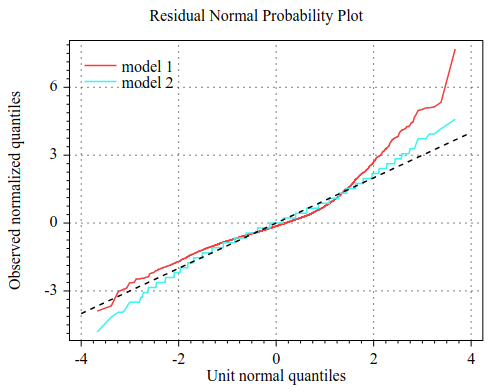
Residual Normal Probability Plot
The Normal Probability Plot on the Residual is a Quantile Quantile Plot between the residual (normalized in variance) and the unit normal distribution.
A straight diagonal normal probability plot is indicative that the residual is normally distributed. If not diagonal, the shape of the plot can be used (alongside the residual histogram) to qualify the nature of the residual distribution.
Following is an example of a residual normal probability plot. The residual of model 2 is more or less normal while the residual of model 1 is not.
Conditional {Ground truth, Prediction, Recall} Plot
The Conditional Plots show the relation between two variables Ground truth, Prediction, and Recall. These plots are useful to understand where the models perform best and where the models perform worst.
Following is an example of three conditional plots. Model 1 performs best for low ground truth values, and model 2 looks random (it is a random predictor).
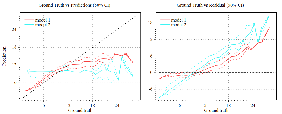
These plots should be read alongside a histogram of the ground truth.
Ranking
We recommend the reading wikipedia page on the learn to rank task.
Normalized Discounted Cumulative Gain (NDCG)
The NDCG is defined as follows:
with:
, \(T\) the truncation (e.g. 5), \(r_i\) the relevance of the i-th example with largest prediction, and \(\hat{r}_i\) is the relevance of the i-th example with largest relevance (i.e. \(\hat{r}_1 \geq \hat{r}_2 \geq \cdots\)).
A popular convention is for the relevance to be a number between 0 and 4, and for the gain function to be \(G(r) = 2^{r_i} - 1\).
The NDCG value is contained between 0 (worst) and 1 (perfect).
In case of ties in the predictions (i.e. the model predicts the same value for two examples), the gain is averaged across the tied elements (see Computing Information Retrieval Performance Measures Efficiently in the Presence of Tied Scores).
The default NDCG is computed by averaging the gain over all the examples.
See section 3 of From RankNet to LambdaRank to LambdaMART: An Overview for more details.
Feature selection
Feature selection algorithms identify and remove unnecessary input features, improving model quality, and speeding up subsequent training. See the Wikipedia article for more details.